Quickfix: Muting search highlights in Emacs Evil mode

This quickfix is about muting search highlights when using the text editor Emacs with its vim emulation Evil mode.

Problem description

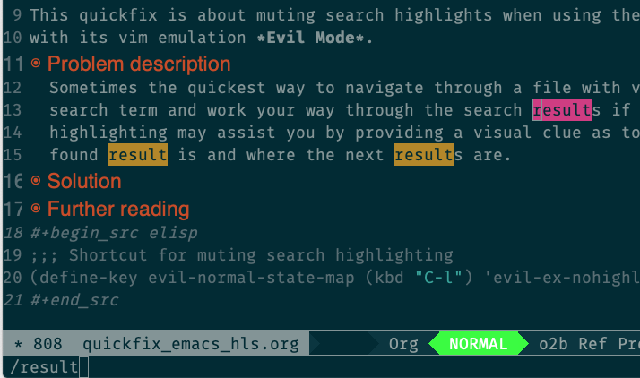
A screenshot of Emacs showing a few highlighted search results.
Search highlighting in Emacs’ Evil mode.

Sometimes the quickest way to navigate through a file with vim is to enter a search term and work your way through the search results if necessary. Search highlighting may assist you by providing a visual clue as to what your current found result is and where the next results are. However, as soon as the cursor is in your desired position, search highlighting persists and can become a nuisance. Fortunately, there is a quick way to mute it on demand: The :noh command (short for :nohlsearch) has exactly this purpose. If you want an even more comfortable solution, you can create a custom shortcut in vim. Drew Neil suggests in Tip 80 of his book Practical Vim to bind the :noh command as an add-on to the key combination Ctrl+l:
  nnoremap <silent> <C-l> :<C-u>nohlsearch<CR><C-l>

This makes sense because Ctrl+l normally redraws the buffer in vim and muting of search highlights is a sensible feature to add. In Emacs, we may do the same and bind Ctrl+l to a macro executing the strokes :noh in evil normal state. However, there is a slightly faster solution available.

Solution

The variable evil-ex-commands, as its name suggests, contains the information which ex command corresponds to which lisp function. A quick call to describe variable (shortcut Ctrl+h Ctrl+v) and a search for “nohl” yield that :noh call the lisp function evil-ex-nohighlight. Thus,

;;; Shortcut for muting search highlighting
(define-key evil-normal-state-map (kbd "C-l") 'evil-ex-nohighlight)

is the desired solution. Note that the standard behavior of Ctrl+l in Emacs is to recenter the viewpoint at bottom, top or original center, a functionality which I personally do not need since Evil mode provides some alternatives (for example, H, M, and L jump to the top, center, and bottom, respectively, of the current buffer and zz centers the current cursor position vertically). However, if you also want to redraw the buffer just like in the vim solution the elisp function redraw-frame seems to do the trick.

;;; Shortcut for redrawing the current frame/buffer and muting search highlighting
(define-key evil-normal-state-map (kbd "C-l") (progn 'redraw-frame 'evil-ex-nohighlight))

Quickfix: Using Lombok with IntelliJ causes compiler error “cannot resolve method”

Quickfixes are short posts that deal with small problems that I encounter and their solutions. This blog post is about a compiler error I stumbled about when using the Java library Lombok in conjunction with the IDE IntelliJ.

Problem description

To understand the problem, we first need to know what the library Lombok is all about.

About Lombok

Lombok is a library that reduces boilerplate code when using the Java programming language. In comparison with modern script languages such as Python or Ruby, Java tends to be overly verbose: In order to create a class with a few attributes serving as a data object, one needs to create numerous getters and setters as well as custom equals and hashCode implementations. Of course, the Java IDE landscape has reacted to this kind of problem a long time ago by equipping IDE users with several ways to generate these methods on demand.

However, maintaining such data classes can still be hassle: Just imagine a programmer quickly adding one or more attributes to a data class because a new feature needs to be implemented that relies on those. They surely will remember to generate the getters and setters because otherwise they won’t be able to access the new attributes. They might miss to update the toString method or the equals and hashCode methods, though, and what gives? All tests might pass and everything could be fine for a while. But then a bug is discovered that either might be related to the equals method not reflecting the newly added attributes that could potentially lead to overwriting data entities in collections or a crucial log message does not give a programmer the values of the added attributes because the toString method has not been updated.

Lombok deals with these problems by generating getters, setters, constructors, useful toString methods as well as equals and hashCode implementations in the build process of your app. Integrating Lombok, say, in a Gradle build, is as easy as adding

compileOnly 'org.projectlombok:lombok'

to the dependencies of your build.gradle file. Afterwards, a data class may be written as follows:

import lombok.*;

@Data
@NoArgsConstructor
@RequiredArgsConstructor
class Account {
  private @NonNull String accNumber;
  private double saldo;
}

The annotation @Data gives you getters and setters for all attributes of your class as well as a toString, a hashCode and an equals implementation. The annotations @NoArgsConstructor and @RequiredArgsConstructor give you the standard constructor as well as a constructor with all the required fields (in this case, all fields annotated as @NonNull).

The problem

Using the data class without further ado in IntelliJ might lead to a compiler error (even though the Gradle build will go through just fine): If we were to use the method setAccNumber, for instance, IntelliJ would remark that it “cannot resolve method setAccNumber“.

The solution

Install the IntelliJ Lombok plugin by searching for “Lombok” in Preferences -> Plugins and hitting install on the first hit. The compiler error should disappear after restarting IntelliJ.

Original Song: Letting Go

In these kinds of blog post I would like to write about my own songs, the idea behind them and the lyrics. I’d like to start with an old song of mine, written over 10 years ago and rearranged about a year ago with the piano as the central element: Letting Go.

About the lyrics

I will keep my dream
And hide it far away
If I ever see that I just cannot find my way
So you stand right there
Behind your wall of thoughts
What will you do when you realize that all roses are made of thorns?
Well, I know all that’s good to me won’t set me free
But, you know I just can’t see the liberty of finally letting go
As the feelings fade
As my eyes seem to open up
I lay my hands on that golden seal and realize it’s just a lock

Lyrics of Letting Go

When I wrote the lyrics, I remember that I was in a situation where a clear cut was objectively the best option to take. But a clear cut also meant to cut something off. I remember being in limbo for a few weeks where I just knew I needed to let go of several things but I was not ready to do so and I could not see the advantage of letting go yet – this is what the line I just can’t see the liberty of finally letting go in the chorus is supposed to emphasize.

The first two verses are some kind of dialogue between the heart (first verse) and reason (second verse). While the heart states that it wants to stay in limbo for a while, hiding and keeping its dreams for the time being because it is unsure of which way to take, reason argues that no matter what way you finally choose, it will not work out without some cuts (all roses are made of thorns).

The third verse is about the necessary change of perspective to finally get out of limbo: The one fundamental truth that must not be touched under all circumstances (the golden seal) turns out to be an obstacle (it’s just a lock). This realization paves the way for the final decision to take action after the last chorus: But I finally let go.

About the music

Musically, letting go wrote itself for the most part. Originally, I composed it on acoustic guitar while I was playing around with a chord progression revolving around the D major chord with different bass tones. I have always liked progressions like D/Dsus2 – D/A – G. This time, however I ended up with Dsus2 – D/A – C which sounded intriguing. I suppose the reason why is that the first two chords establish a D major feeling that is destroyed by the C chord. After two repetitions, the progression goes on to resolve to G.

This leaves us with two home bases for the composition: While D and D/A hint at the piece being written in D major, C and G hint at a composition in G major. And actually, that’s all there is to it. The conflict conjured up by the lyrics is simply reflected by the composition. Indeed, while we know that D major is a more natural key for this piece (we end up with an Asus4 / A chord at the end of each verse), the C major chord plays a prominent part the entire time.

In fact, the final repetition of the chorus ends on a C major chord before we finally let go of it and end the piece on D major.

Means and medians

Understanding random experiments through deterministic invariants is a central goal of the mathematical branch known as probability theory or stochastics. While the expected value (or the mean) of a random experiment has a very natural interpretation (as its name suggests, it is the value we expect to occur on average when repeating the experiment) and a simple ad hoc definition as well as an easy generalization once foundations of measure theory have been established, the situation for the median is not as nice. Even though the median is more robust when dealing with outliers and, thus, might yield a more convenient substitute for the expected value, I have not encountered a general definition and treatment of it until I was concerned with learning the underlying statistical theory of Machine Learning (as for instance in The Elements of Machine Learning by Hastie et. al. or in Understanding Machine Learning: From Theory to Algorithms by Shalev-Shwartz and Ben-David). This post gives a basic treatment for discrete random variables and should be accessible to readers with some understanding of elementary discrete math and probability.

Expected values and medians for discrete random variables

Let $latex X$ be a random variable attaining finitely many real values $latex \{x_1, \dotsc, x_k\} \subset \mathbf{R}$. Denote the probability that $latex X = x_i$ by $latex p_i$. We know that

  • $latex 0 \leq p_i \leq 1$ for all $latex i$ and
  • $latex \sum_{i=1}^k p_i = p_1 + p_2 + \dotsc + p_k = 1.$

Definition. The expected value (or the mean) of the random variable $latex X$, denoted by $latex \mathbb{E}[X]$ is the weighted average of its values, weighted by their respective probabilities, i.e. $latex \mathbb{E}[X] := \sum_{i=1}^k p_i x_i.$

Let us quickly discuss a couple of examples and some computational rules before moving on to the median.

  • If \(X\) is constant, i.e. it only attains one value \(x_1\) with probability \(p_1 = 1\), then the expected value agrees with that one value.
  • If we assume that $latex p_1 = \dotsc = p_k = 1/k$, i.e. that $latex X$ is distributed uniformly on its values, then the expected value will be the ordinary average of the values $latex \{x_1, \dotsc, x_k\}$.
  • Let $latex k = 2$ so that $latex X$ takes on only two values. Let the first value be $latex x_1 = 0$ taken on with probability $latex p_1 = 0.9999$ and let the second value be $latex x_2 = 10000000000 = 10^{10}$ taken on with probability $latex p_2 = 1 – p_1 = 0.0001 = 10^{-4}$. By our definition, the expected value of $latex X$ is \begin{align*}\mathbb{E}[X] &= p_1 x_1 + p_2 x_2 \\&= 0.999 \cdot 0 + 10^{-4} \cdot 10^{10} = 10^6.\end{align*} Even though we know with 99.99% probability that $latex X$ will be zero, the expected value is some unexpectedly high number because there is the trace of a chance that $latex X = 10^{10}$. This example is the heart of what we mean by that the expected value is prone to outliers.

Computational rules. The following rules are central to the expected value. They may be proved by (more or less) direct computation from the definition.

  • The expected value is monotone, i.e. for random variables $latex X, Y$ such that $latex X \geq Y$, we also have $latex \mathbb{E}[X] \geq \mathbb{E}[Y]$.
  • The expected value is a linear functional, i.e. for real numbers $latex \alpha, \beta \in \mathbb{R}$ and another random variable $latex Y$, $latex \mathbb{E}[\alpha X + \beta Y] = \alpha\mathbb{E}[X] + \beta\mathbb{E}[Y]$.

Definition. A median of the random variable $latex X$ denoted by $latex \mathbb{M}[X]$ or $latex \mathbf{Median}[X]$ is a real number such that both the probabilities that $latex X \leq \mathbb{M}[X]$ as well as $latex X \geq \mathbb{M}[X]$ are bigger than $latex 1/2$. In formulae: $latex P(X \leq \mathbb{M}[X]) \geq 1/2$ and $latex P(X \geq \mathbb{M}[X]) \geq 1/2$.

The problem is immediately apparent: The definition does not give a formula for the median and there is no reason for the median to be unique (note that I only defined what a median is). Let us take a look at the same examples we exercised for the expected value.

  • If \(X\) is constant then the median agrees with the value that \(X\) attains with probability \(1\). Even this trivial example is not as immediate as in the case of the expected value, so let’s give some details: Let’s say the sole value that \(X\) attains is \(x\). Then we certainly have \(P(X \geq x) = 1 \geq 1/2\) and \(P(X \leq x) = 1 \leq 1/2\).
  • If $latex X$ is distributed uniformly on its values, we may compute the median by ordering its values. Let $latex x_1 < \dotsb < x_k$ be such an ordering of its values. We claim that every real number in the closed interval $latex I = [x_{\lfloor(k+1)/2\rfloor}, x_{\lceil(k+1)/2\rceil}]$ is a median of $latex X$. Here, $latex \lfloor(k+1)/2\rfloor$ denotes the biggest integer smaller than $latex (k+1)/2$ and $latex \lceil(k+1)/2\rceil$ denotes the smallest integer bigger than $latex (k+1)/2$ (in German, these brackets are known as the lower resp. upper Gauß brackets). If $latex k$ is odd, $latex (k+1)/2$ already is an integer. In this case, $latex I$ consists of one single point. Now, let $latex x \in I$. Then $latex x \geq x_{\lfloor(k+1)/2\rfloor}$ and, thus, \begin{align*} P(X \leq x) &\geq P(X \leq x_{\lfloor(k+1)/2\rfloor})\\ &= p_1 + \dotsb + p_{\lfloor(k+1)/2\rfloor} \\ &= 1/k (\lfloor(k+1)/2\rfloor) \\ &\geq 1/k ( (k+1)/2 – 1/2) = 1/2. \end{align*} The other defining inequality follows similarly. Often, the median is agreed to be the middle point of the interval $latex I$ so that one can talk about the median in this case.
  • Let \(X\) be the random variable taking on the value $latex 0$ with probability $latex 0.9999$ and $latex 10^{10}$ with probability $latex 10^{-4}$. Then $latex \mathbb{M}[X] = 0$ is the only median of $latex X$. Indeed, $latex P(X \geq 0) = 1 \geq 1/2$ and $latex P(X \leq 0) = P(X = 0) = 0.9999 \geq 1/2$ so that $latex 0$ is a median of $latex X$. If $latex x > 0$, then $latex P(X \geq x) = 10^{-4} < 1/2$ and if $latex x < 0$, then $latex P(X \leq x) = 0 < 1/2$ so that in both cases $latex x$ cannot be a median of $latex X$.

Comparing the outcome of the last example for the expected value and the median, we see that the median yields a more typical value of the random variable if its distribution is skewed. What if the distribution is symmetric, though?

Definition. Let $latex X$ be a random variable. We say that $latex X$ is distributed symmetrically onto its values if there is a symmetry point, i.e., a real value $latex s$ such that $latex P(X \geq s + x) = P(X \leq s – x)$ for all real values $latex x$.

Observation. If $latex X$ is distributed symmetrically onto its values, then the expected value is a median, i.e. $latex \mathbb{E}[X] = \mathbb{M}[X]$.

I would like to prove this observation; actually, I would like to do a little more and give you some insight into the thought process that goes into writing a proof for this. In order to separate my thought process from the sentences that actually end up being written up in the proof, let us agree on this: My thought process will be written in normal weight, while sentences in the proof will be written in cursive. This should come as no surprise, as more often than not proofs tend to be written in dense, short language without any decoration, but let me give you a spoiler here: Much more will be spent on elaborating on my thought process than actually writing down the proof.

Proof. We start with one thing that mathematicians often do to make the proof more readable. We write “without loss of generality we may assume…”, followed by a replacement of the original statement in question with something that, at first, might seem like a special case.

Let me give you more details for the statement at hand. I would like to get rid of the nuisance that is the existence of the symmetry point in the definition of a symmetric distribution. What if I were to replace the random variable $latex X$ by $latex Y = X – s$? Well, this shifts the values: $latex Y$ takes on the values $latex y_1 < \dotsb < y_k$ where $latex y_i = x_i – s$. And this makes $latex 0$ a symmetry point for its values; indeed, \begin{align*}P(Y \geq 0 + x) &= P(X – s \geq x) = P(X \geq s + x) \\ &= P(X \leq s-x) = P(Y \leq 0-x).\end{align*}Okay, this means that we have replaced $latex X$, the random variable that has some unknown symmetry point $latex s$, by some special random variable $latex Y$ that has a symmetry point $latex 0$ that looks like it could be easier to handle. But what about our task at hand? Let us assume that we have proven the statement for the random variable $latex Y$, i.e., that the expected value $latex \mathbb{E}[Y]$ is a median of $latex Y$. Does this tell us something about $latex X$? Yes: since $latex Y = X – s$ and because the expected value is linear, we have $latex \mathbb{M}[X-s] = \mathbb{M}[Y] = \mathbb{E}[Y] = \mathbb{E}[X-s] = \mathbb{E}[X] – s$. We are close. If we knew that $latex \mathbb{M}[X-s] = \mathbb{M}[X] – s$, it would immediately follow that the expected value of $latex X$ is a median. And, in fact, this holds: Let $latex m$ be a median of $latex X$. Then \(P(X-s \geq m-s) = P(X \geq m) \geq 1/2\) and \(P(X-s \leq m-s) = P(X \leq m) \geq 1/2.\)

This all means that it is sufficient to prove the statement for the special random variable $latex Y$ because, as we have shown above, this implies that the statement is also true for $latex X$. Because mathematicians do not like to waste letters (or, rather, we like the letter $latex X$ quite a lot), we tend to rename $latex Y$ and call it $latex X$ again. Still with me? We are ready to write the first sentence of our proof:

Without loss of generality, we may assume that $latex X$ has $latex 0$ as its symmetry point.

More often than not, there is no justification given for why no generality has been lost, because after all that internal monologue that led to this sentence it should be obvious (at least to the author). Because we might feel pity on any future reader stumbling upon this first sentence, let us at least leave a small hint for why this replacement is sane:

Without loss of generality, we may assume that $latex X$ has $latex 0$ as its symmetry point (otherwise, replace $latex X$ by $latex X – s$ where $latex s$ is the original symmetry point).

One fact should be emphasized here: A written mathematical proof should not be expected to spell out every small detail to the reader. Rather, a proof should be a blueprint or a guideline that assists the reader in gaining understanding of why the statement is true. How much detail is spelled out depends on the mathematical level of the text the proof is embedded in. It is very much possible that the observation we are proving right now is left as an exercise to the reader if we are reading a text book on advanced probability theory or statistics so that the reader is expected to have some background on those topics.

Okay, let us turn to some computations now. Because the condition on the probabilities in the definition of a symmetric distribution and in the definition of the median look quite similar, let’s try and compute the median first. Since we have assumed that $latex 0$ is a symmetry point and the condition $latex P(X \geq x) = P(X \leq -x)$ holds for all real values $latex x$, it has to hold for $latex 0$, which means $latex P(X \geq 0) = P(X \leq 0)$. This looks like it could be useful if we were to prove that $latex 0$ is a median. Let’s see: Because $latex X$ is a real valued random variable, the probability that $latex X$ attains any real value is $latex 1$ (otherwise, something would be very off). We could rephrase that by saying that $latex X$ either is a negative real number, or a non-negative real number. Let us write this down in formulas: $latex 1 = P(X \geq 0 \text{ or } X < 0) = P(X \geq 0) + P(X < 0)$. Here, we have used that the events “$latex X$ is negative” and “$latex X$ is non-negative” are disjoint so that their probabilites simply add up to the union. Since the probability that $latex X$ is negative is smaller than or equal to the probability that $latex X$ is non-positive (because potentially $latex 0$ could be a value $latex X$ attains), we see that $latex P(X < 0) \leq P(X \leq 0)$. Putting this together with the assumption that $latex P(X \leq 0) = P(X \geq 0)$, we obtain $latex 1 \leq P(X \geq 0) + P(X \leq 0) = 2P(X\geq 0)$, i.e. that $latex P(X \leq 0) = P(X \geq 0) \geq 1/2)$ so that $latex 0$ is a median. This lays down a proof strategy: We may show the assertion somewhat indirectly, namely by showing that both the median and the mean are $latex 0$. Let us write this down to prepare our reader for the following.

We will show that both the median and the expected value are $latex 0$.

Since we have already worked out that the median is $latex 0$, we may pin that down.

We will start by showing that the median is $latex 0$.

Now, to write computations down more concisely, mathematicians tend to rewrite their whole thought process in reverse order in a single string of equations leading to the desired result. Let me show you how this could be done in this case.

Since $latex 0$ is a symmetry point, we have \begin{align*}P(X \leq 0) &= P(X \geq 0) \\ &= 1/2 \bigl(P(X \geq 0) + P(X \leq 0)\bigr) \\ &\geq 1/2 \bigl( P(X \geq 0) + P(X < 0)\bigr) = 1/2\end{align*} which shows that $latex 0$ is a median.

A reader well-versed in basic probability theory can immediately follow these computations so that we leave out any justifications.

Turning to the expected value, we could use its definition and the assumption on the random value but I’m not exactly sure how. Also, my guts tell me that this will be a mess of indices and intransparent computation. Maybe a more abstract argument will work here. Let’s rephrase the fact that \(0\) is a symmetry point slightly: For each real value \(x\) we have \(P(X \leq x) = P(X \geq -x) = P(-X \leq x).\) This means that the functions \(x \mapsto F_X(x) := P(X \leq x)\) and \(x \mapsto F_{-X}(x) := P(-X \leq x)\) agree everywhere. These functions are known as the distribution function of \(X\) resp. \(-X\) and, as their name suggests, encode information about the way a random variable is distributed. This suggests that \(X\) and \(-X\) are identically distributed, i.e. they attain the same values with the same probabilities and this of course means that they share the same expected value. And this is precisely what we need: Because the expected value is linear, \[\mathbb{E}[X] = \mathbb{E}[-X] = -\mathbb{E}[X].\] But this is only possible if \(\mathbb{E}[X] = 0\). If you have never heard of distribution functions before, let me give some hints for how to show that \(X\) and \(-X\) share the same values attained with the same probabilities more directly. Order the values \(x_1 < \dotsb < x_k\) of \(X\). Then for \(x < x_1\), \[P(-X \leq x) = P(X \leq x) = 0.\] This means that \(x_1\) is the smallest value that both \(X\) and \(-X\) attain. And they attain it with equal probability since \[P(-X \leq x_1) = P(X \leq x_1) = p_1.\] Now we can work our way up through the values of \(X\) inductively. If we have already shown that both \(X\) and \(-X\) attain the values \(x_1, \dotsc, x_i\) with the same probability, then \[P(-X \leq x) = P(X \leq x) = p_1 + \dotsb + p_i\] for all \(x_i \leq x < x_{i+1}\) which means that there is no value in between \(x_i\) and \(x_{i+1}\) that \(-X\) attains. And \(-X\) attains \(x_{i+1}\) with probability \(p_{i+1}\) since \[P(-X \leq x_{i+1}) = P(X \leq x_{i+1}) = p_1 + \dotsb + p_{i+1}.\] Okay, now let’s see what ends up being written in the proof:

Turning to the expected value, a rephrasing of \(0\) begin a symmetry point is that \(P(X \leq x) = P(X \geq -x) = P(-X \leq x)\) which means that \(X\) and \(-X\) share the same distribution function. Since this implies that they both attain the same values with the same probability, we have \(\mathbb{E}[X] = \mathbb{E}[-X] = -\mathbb{E}[X]\) so that \(\mathbb{E}[X] = 0\) follows.

Up to now, one could come to the conclusion that a random variable is far from being symmetrically distributed if the expected value and the median stray far from each other (especially when recalling the example with the huge outlier). However, this is not the case. Let us look at a modification of the example with the huge outlier.

Example. Let \(X\) be a random variable attaining the values \(\{0, 10^{10}\}\). Assume that \(0\) is attained with probability \(1/2 + \varepsilon\) where \(\varepsilon > 0\) is some arbitrarily small positive number. Then \(\mathbb{M}[X] = 0\) while \[\mathbb{E}[X] = (1/2 – \varepsilon) 10^{10} \geq 10^9\] at least for \(\varepsilon \leq 2/5\).

The last example shows that the strength of the median is also its weakness: The median only factors in the majority of values a random variable attains even if the majority is only ever-so-slightly bigger than \(1/2\). One fix could be to not only consider the median but also the first and the third quartile: These are real values that split up the values a random variable attains differently; namely, the first quartile \(q_1\) is a real value such that \(P(X \leq q_1) \geq 0.25\) and \(P(X \geq q_1) \geq 0.75\) while the third quartile satisfies \(P(X \leq q_3) \geq 0.75\) and \(P(X \geq q_3) \geq 0.25\). In this context, the median is also known as the second quartile. Even more generally, we could extract the follow invariant.

Definition. Let \(0 \leq \delta \leq 1\) and \(X\) be a random variable. A \(\delta\)-quantile for the random variable \(X\) is a real number \(q_\delta\) such that \(P(X \leq q_\delta) \geq \delta\) and \(P(X \geq q_\delta) \geq 1 – \delta.\)

Thus, the median may also be called a \(1/2\)-quantile. A warning: The notation here might not be standard; for instance, the wikipedia article about quantiles (https://en.wikipedia.org/wiki/Quantile) talks about \(k\)-th \(q\)-quantiles which we would simply refer to as \(k/q\)-quantiles.

Conclusion. The combination of both invariants gives us a first impression of how well-behaved the distribution is: On the one hand, both the expected value and the median being close to each other might suggest that the distribution is close to being symmetric; on the other hand, both straying far from each other hints at the random variable suffering from outliers. To be sure about this, one should also consider other quantiles.